Image Classification with Vision Transformers
This notebook is largely inspired by the Keras code example Image classification with Vision Transformer by Khalid Salama.
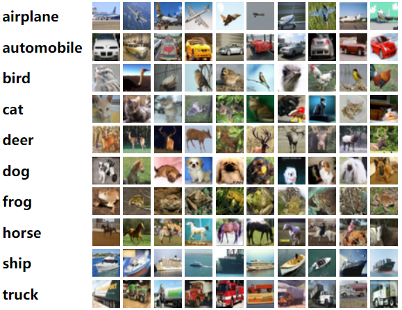
In this example, we will classify images in the CIFAR-10 dataset using the Vision Transformer (ViT) model by Alexey Dosovitskiy et al. using Keras-MML layers.
Important
We will be using some plotting utilities for this notebook. Run the command below to install them, then reload the kernel.
%pip install matplotlib~=3.9.0 seaborn~=0.13.2
Requirement already satisfied: matplotlib~=3.9.0 in /usr/local/lib/python3.10/dist-packages (3.9.1)
Requirement already satisfied: seaborn~=0.13.2 in /usr/local/lib/python3.10/dist-packages (0.13.2)
Requirement already satisfied: contourpy>=1.0.1 in /usr/local/lib/python3.10/dist-packages (from matplotlib~=3.9.0) (1.2.1)
Requirement already satisfied: cycler>=0.10 in /usr/local/lib/python3.10/dist-packages (from matplotlib~=3.9.0) (0.12.1)
Requirement already satisfied: fonttools>=4.22.0 in /usr/local/lib/python3.10/dist-packages (from matplotlib~=3.9.0) (4.53.0)
Requirement already satisfied: kiwisolver>=1.3.1 in /usr/local/lib/python3.10/dist-packages (from matplotlib~=3.9.0) (1.4.5)
Requirement already satisfied: numpy>=1.23 in /usr/local/lib/python3.10/dist-packages (from matplotlib~=3.9.0) (1.23.5)
Requirement already satisfied: packaging>=20.0 in /usr/local/lib/python3.10/dist-packages (from matplotlib~=3.9.0) (24.1)
Requirement already satisfied: pillow>=8 in /usr/local/lib/python3.10/dist-packages (from matplotlib~=3.9.0) (9.4.0)
Requirement already satisfied: pyparsing>=2.3.1 in /usr/local/lib/python3.10/dist-packages (from matplotlib~=3.9.0) (3.1.2)
Requirement already satisfied: python-dateutil>=2.7 in /usr/local/lib/python3.10/dist-packages (from matplotlib~=3.9.0) (2.8.2)
Requirement already satisfied: pandas>=1.2 in /usr/local/lib/python3.10/dist-packages (from seaborn~=0.13.2) (2.0.3)
Requirement already satisfied: pytz>=2020.1 in /usr/local/lib/python3.10/dist-packages (from pandas>=1.2->seaborn~=0.13.2) (2023.4)
Requirement already satisfied: tzdata>=2022.1 in /usr/local/lib/python3.10/dist-packages (from pandas>=1.2->seaborn~=0.13.2) (2024.1)
Requirement already satisfied: six>=1.5 in /usr/local/lib/python3.10/dist-packages (from python-dateutil>=2.7->matplotlib~=3.9.0) (1.16.0)
Set up plotting utilities.
import matplotlib.pyplot as plt
import seaborn as sns

sns.set_theme()
Note
We will use the jax backend for faster execution of the code. Feel free to ignore the cell below.
import os

os.environ["KERAS_BACKEND"] = "jax"
Preparing the Data
Conveniently, the CIFAR-10 dataset is already available in Keras, so we just need to load it from there.
import keras

(x_train, y_train), (x_test, y_test) = keras.datasets.cifar10.load_data()
Note
For faster execution of the code, we will only use 1% of the full dataset (both training and testing). In practice the full training/testing dataset should be used.
DEMO_SPLIT = 0.01

x_train = x_train[: int(x_train.shape[0] * DEMO_SPLIT)]
y_train = y_train[: int(y_train.shape[0] * DEMO_SPLIT)]
x_test = x_test[: int(x_test.shape[0] * DEMO_SPLIT)]
y_test = y_test[: int(y_test.shape[0] * DEMO_SPLIT)]
Let’s take a look at the shapes of the downloaded arrays.
print(f"x_train shape: {x_train.shape} - y_train shape: {y_train.shape}")
print(f"x_test shape: {x_test.shape} - y_test shape: {y_test.shape}")
x_train shape: (500, 32, 32, 3) - y_train shape: (500, 1)
x_test shape: (100, 32, 32, 3) - y_test shape: (100, 1)
The CIFAR-10 dataset contains 10 distinct classes. Each image in the dataset is \(32 \times 32\) with 3 channels, meaning that the INPUT_SHAPE for our model is (32, 32, 3).
NUM_CLASSES = 10
INPUT_SHAPE = (32, 32, 3)
For actual processing, let’s resize the images so that we get more patches that the ViT learns from.
IMAGE_SIZE = 72
To improve the performance of the model, let’s perform some data augmentation on the images.
from keras import layers

data_augmentation = keras.Sequential(
    [
        layers.Normalization(),
        layers.Resizing(IMAGE_SIZE, IMAGE_SIZE),
        layers.RandomFlip("horizontal"),
        layers.RandomRotation(factor=0.02),
        layers.RandomZoom(height_factor=0.2, width_factor=0.2),
    ],
    name="data_augmentation",
)

# Compute the mean and the variance of the training data for normalization
data_augmentation.layers[0].adapt(x_train)
Model Creation
import keras_mml
Let’s define the size of the patches that we want.
PATCH_SIZE = 6
NUM_PATCHES = (IMAGE_SIZE // PATCH_SIZE) ** 2
Let’s display the patches for a sample image. This is done through the Patches layer.
import numpy as np
from keras import ops

plt.figure(figsize=(4, 4))
image = x_train[123]  # Just as an example
plt.imshow(image.astype("uint8"))
plt.axis("off")

resized_image = ops.image.resize(
    ops.convert_to_tensor([image]), size=(IMAGE_SIZE, IMAGE_SIZE)
)
patches = keras_mml.layers.Patches(PATCH_SIZE)(resized_image) #  Patch generation layer
print(f"Image size: {IMAGE_SIZE} X {IMAGE_SIZE}")
print(f"Patch size: {PATCH_SIZE} X {PATCH_SIZE}")
print(f"Patches per image: {patches.shape[1]}")
print(f"Elements per patch: {patches.shape[-1]}")

n = int(np.sqrt(patches.shape[1]))
plt.figure(figsize=(4, 4))
for i, patch in enumerate(patches[0]):
    ax = plt.subplot(n, n, i + 1)
    patch_img = ops.reshape(patch, (PATCH_SIZE, PATCH_SIZE, 3))  # Make it back into RGB
    plt.imshow(ops.convert_to_numpy(patch_img).astype("uint8"))
    plt.axis("off")
Image size: 72 X 72
Patch size: 6 X 6
Patches per image: 144
Elements per patch: 108


To generate the embeddings for the patches, we can use the PatchEmbedding layer that was also included in Keras-MML. This layer will encode each patch as a PROJECTION_DIM-dimensional vector that can be used in the transformer block that is incoming.
PROJECTION_DIM = 64
We are now ready to create the full model. We will use the TRANSFORMER_LAYERS hyperparameter to specify the number of transformer blocks to use in the ViT.
TRANSFORMER_LAYERS = 8
NUM_HEADS = 4
model = keras.models.Sequential()
model.add(layers.Input(shape=INPUT_SHAPE))

# Augment the data
model.add(data_augmentation)

# Create patches
model.add(keras_mml.layers.Patches(PATCH_SIZE))

# Create patch embeddings
model.add(keras_mml.layers.PatchEmbedding(NUM_PATCHES, PROJECTION_DIM, with_positions=True))

# Use multiple transformer blocks
for _ in range(TRANSFORMER_LAYERS):
    model.add(keras_mml.layers.TransformerBlockMML(PROJECTION_DIM, PROJECTION_DIM * 2, NUM_HEADS, rate=0.1))

# Normalize, flatten, and dropout
model.add(layers.LayerNormalization(epsilon=1e-6))
model.add(layers.Flatten())
model.add(layers.Dropout(0.5))

# Add SwiGLUMML for final classification fine tuning
model.add(keras_mml.layers.DenseMML(1024))
model.add(keras_mml.layers.DenseMML(256))

# Final classification head
model.add(layers.Dense(NUM_CLASSES))

model.summary()
Model: "sequential"
┏━━━━━━━━━━━━━━━━━━━━━━━━━━━━━━━━━━━━━━┳━━━━━━━━━━━━━━━━━━━━━━━━━━━━━┳━━━━━━━━━━━━━━━━━┓
┃ Layer (type)                         ┃ Output Shape                ┃         Param # ┃
┡━━━━━━━━━━━━━━━━━━━━━━━━━━━━━━━━━━━━━━╇━━━━━━━━━━━━━━━━━━━━━━━━━━━━━╇━━━━━━━━━━━━━━━━━┩
│ data_augmentation (Sequential)       │ (None, 72, 72, 3)           │               7 │
├──────────────────────────────────────┼─────────────────────────────┼─────────────────┤
│ patches_1 (Patches)                  │ (None, 144, 108)            │               0 │
├──────────────────────────────────────┼─────────────────────────────┼─────────────────┤
│ patch_embedding (PatchEmbedding)     │ (None, 144, 64)             │          31,744 │
├──────────────────────────────────────┼─────────────────────────────┼─────────────────┤
│ transformer_block_mml                │ (None, 144, 64)             │          69,440 │
│ (TransformerBlockMML)                │                             │                 │
├──────────────────────────────────────┼─────────────────────────────┼─────────────────┤
│ transformer_block_mml_1              │ (None, 144, 64)             │          69,440 │
│ (TransformerBlockMML)                │                             │                 │
├──────────────────────────────────────┼─────────────────────────────┼─────────────────┤
│ transformer_block_mml_2              │ (None, 144, 64)             │          69,440 │
│ (TransformerBlockMML)                │                             │                 │
├──────────────────────────────────────┼─────────────────────────────┼─────────────────┤
│ transformer_block_mml_3              │ (None, 144, 64)             │          69,440 │
│ (TransformerBlockMML)                │                             │                 │
├──────────────────────────────────────┼─────────────────────────────┼─────────────────┤
│ transformer_block_mml_4              │ (None, 144, 64)             │          69,440 │
│ (TransformerBlockMML)                │                             │                 │
├──────────────────────────────────────┼─────────────────────────────┼─────────────────┤
│ transformer_block_mml_5              │ (None, 144, 64)             │          69,440 │
│ (TransformerBlockMML)                │                             │                 │
├──────────────────────────────────────┼─────────────────────────────┼─────────────────┤
│ transformer_block_mml_6              │ (None, 144, 64)             │          69,440 │
│ (TransformerBlockMML)                │                             │                 │
├──────────────────────────────────────┼─────────────────────────────┼─────────────────┤
│ transformer_block_mml_7              │ (None, 144, 64)             │          69,440 │
│ (TransformerBlockMML)                │                             │                 │
├──────────────────────────────────────┼─────────────────────────────┼─────────────────┤
│ layer_normalization                  │ (None, 144, 64)             │             128 │
│ (LayerNormalization)                 │                             │                 │
├──────────────────────────────────────┼─────────────────────────────┼─────────────────┤
│ flatten (Flatten)                    │ (None, 9216)                │               0 │
├──────────────────────────────────────┼─────────────────────────────┼─────────────────┤
│ dropout_16 (Dropout)                 │ (None, 9216)                │               0 │
├──────────────────────────────────────┼─────────────────────────────┼─────────────────┤
│ dense_mml_17 (DenseMML)              │ (None, 1024)                │       9,447,424 │
├──────────────────────────────────────┼─────────────────────────────┼─────────────────┤
│ dense_mml_18 (DenseMML)              │ (None, 256)                 │         263,424 │
├──────────────────────────────────────┼─────────────────────────────┼─────────────────┤
│ dense (Dense)                        │ (None, 10)                  │           2,570 │
└──────────────────────────────────────┴─────────────────────────────┴─────────────────┘
Total params: 10,300,817 (39.29 MB)
Trainable params: 10,300,810 (39.29 MB)
Non-trainable params: 7 (28.00 B)
We compile the model, using the Adam optimizer with weight decay (i.e., AdamW) and aiming to minimize the sparse categorical crossentropy. We monitor the accuracy and top-5 accuracy scores.
from keras import optimizers, losses, metrics

model.compile(
    optimizer=optimizers.AdamW(learning_rate=1e-3, weight_decay=1e-4),
    loss=losses.SparseCategoricalCrossentropy(from_logits=True),
    metrics=[
        metrics.SparseCategoricalAccuracy(name="acc"),
        metrics.SparseTopKCategoricalAccuracy(5, name="top_5_acc"),
    ],
)
We will also regularly save the weights of the model, and keeping only the weights that make the model score the highest in the validation accuracy.
from keras import callbacks

checkpoint_filepath = "misc/vit/checkpoint.weights.h5"
checkpoint_callback = callbacks.ModelCheckpoint(
    checkpoint_filepath,
    monitor="val_acc",
    save_best_only=True,
    save_weights_only=True,
)
We can now train the model.
history = model.fit(
    x_train,
    y_train,
    batch_size=32,
    epochs=5,  # We use 5 epochs here for demonstration purposes. Use somewhere around 100 epochs for real training
    validation_split=0.1,
    callbacks=[checkpoint_callback],
)
Epoch 1/5
15/15 ━━━━━━━━━━━━━━━━━━━━ 235s 15s/step - acc: 0.1486 - loss: 4.6825 - top_5_acc: 0.5412 - val_acc: 0.2000 - val_loss: 4.3141 - val_top_5_acc: 0.7000
Epoch 2/5
15/15 ━━━━━━━━━━━━━━━━━━━━ 200s 13s/step - acc: 0.2015 - loss: 3.5198 - top_5_acc: 0.7247 - val_acc: 0.2600 - val_loss: 2.3203 - val_top_5_acc: 0.6400
Epoch 3/5
15/15 ━━━━━━━━━━━━━━━━━━━━ 163s 11s/step - acc: 0.2339 - loss: 2.2447 - top_5_acc: 0.7672 - val_acc: 0.1800 - val_loss: 2.2486 - val_top_5_acc: 0.7400
Epoch 4/5
15/15 ━━━━━━━━━━━━━━━━━━━━ 205s 14s/step - acc: 0.2787 - loss: 1.9467 - top_5_acc: 0.8139 - val_acc: 0.3600 - val_loss: 2.0642 - val_top_5_acc: 0.8200
Epoch 5/5
15/15 ━━━━━━━━━━━━━━━━━━━━ 167s 11s/step - acc: 0.3966 - loss: 1.7190 - top_5_acc: 0.8764 - val_acc: 0.2800 - val_loss: 2.1091 - val_top_5_acc: 0.8200
Let’s see how good the model is on the test dataset.
model.load_weights(checkpoint_filepath)
_, accuracy, top_5_accuracy = model.evaluate(x_test, y_test)
print(f"Test accuracy: {accuracy * 100:.2f}%")
print(f"Test top 5 accuracy: {top_5_accuracy * 100:.2f}%")
4/4 ━━━━━━━━━━━━━━━━━━━━ 13s 3s/step - acc: 0.3947 - loss: 1.8359 - top_5_acc: 0.8494
Test accuracy: 38.00%
Test top 5 accuracy: 85.00%
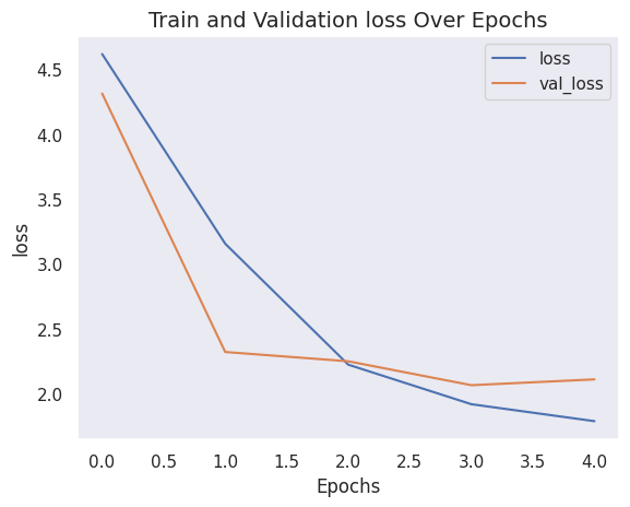
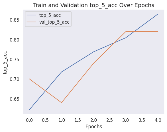
What does the model’s history look like?
def plot_history(item):
    plt.plot(history.history[item], label=item)
    plt.plot(history.history["val_" + item], label="val_" + item)
    plt.xlabel("Epochs")
    plt.ylabel(item)
    plt.title(f"Train and Validation {item} Over Epochs", fontsize=14)
    plt.legend()
    plt.grid()
    plt.show()
plot_history("loss")
plot_history("top_5_acc")
Conclusion
After 5 epochs, the ViT model achieves around 38% accuracy and 85% top-5 accuracy on the test data. These are not competitive results on the CIFAR-10 dataset. Certainly, this could be due to the small sample used for training in this demonstration, but the more important reason is that this is not how the ViT paper performs the training.
The state of the art results reported in the paper are achieved by pre-training the ViT model using the JFT-300M dataset, then fine-tuning it on the target dataset (i.e. the CIFAR-10 dataset). In practice, it’s recommended to fine-tune a ViT model that was pre-trained using a large, high-resolution dataset.
Regardless, we used mostly matmul-less layers in this model, and we still achieved commendable results.