Time Series Forecasting
This notebook is largely inspired from Jason Brownlee’s LSTM time series prediction article on Machine Learning Mastery.
In this example, we will do time series forecasting using Keras-MML’s Gated Recurrent Unit (GRU) and Linear Recurrent Unit (LRU) implementations.
Important
We will be using some dataset processing and plotting utilities for this notebook. Run the command below to install them, then reload the kernel.
%pip install pandas~=2.2.2 scikit-learn~=1.5.0 matplotlib~=3.9.0 seaborn~=0.13.2
Requirement already satisfied: pandas~=2.2.2 in /home/vscode/.cache/pypoetry/virtualenvs/keras-matmulless-b9IALFmu-py3.10/lib/python3.10/site-packages (2.2.2)
Requirement already satisfied: scikit-learn~=1.5.0 in /home/vscode/.cache/pypoetry/virtualenvs/keras-matmulless-b9IALFmu-py3.10/lib/python3.10/site-packages (1.5.0)
Requirement already satisfied: matplotlib~=3.9.0 in /home/vscode/.cache/pypoetry/virtualenvs/keras-matmulless-b9IALFmu-py3.10/lib/python3.10/site-packages (3.9.0)
Requirement already satisfied: seaborn~=0.13.2 in /home/vscode/.cache/pypoetry/virtualenvs/keras-matmulless-b9IALFmu-py3.10/lib/python3.10/site-packages (0.13.2)
Requirement already satisfied: numpy>=1.22.4 in /home/vscode/.cache/pypoetry/virtualenvs/keras-matmulless-b9IALFmu-py3.10/lib/python3.10/site-packages (from pandas~=2.2.2) (1.26.4)
Requirement already satisfied: python-dateutil>=2.8.2 in /home/vscode/.cache/pypoetry/virtualenvs/keras-matmulless-b9IALFmu-py3.10/lib/python3.10/site-packages (from pandas~=2.2.2) (2.9.0.post0)
Requirement already satisfied: pytz>=2020.1 in /home/vscode/.cache/pypoetry/virtualenvs/keras-matmulless-b9IALFmu-py3.10/lib/python3.10/site-packages (from pandas~=2.2.2) (2024.1)
Requirement already satisfied: tzdata>=2022.7 in /home/vscode/.cache/pypoetry/virtualenvs/keras-matmulless-b9IALFmu-py3.10/lib/python3.10/site-packages (from pandas~=2.2.2) (2024.1)
Requirement already satisfied: scipy>=1.6.0 in /home/vscode/.cache/pypoetry/virtualenvs/keras-matmulless-b9IALFmu-py3.10/lib/python3.10/site-packages (from scikit-learn~=1.5.0) (1.13.1)
Requirement already satisfied: joblib>=1.2.0 in /home/vscode/.cache/pypoetry/virtualenvs/keras-matmulless-b9IALFmu-py3.10/lib/python3.10/site-packages (from scikit-learn~=1.5.0) (1.4.2)
Requirement already satisfied: threadpoolctl>=3.1.0 in /home/vscode/.cache/pypoetry/virtualenvs/keras-matmulless-b9IALFmu-py3.10/lib/python3.10/site-packages (from scikit-learn~=1.5.0) (3.5.0)
Requirement already satisfied: contourpy>=1.0.1 in /home/vscode/.cache/pypoetry/virtualenvs/keras-matmulless-b9IALFmu-py3.10/lib/python3.10/site-packages (from matplotlib~=3.9.0) (1.2.1)
Requirement already satisfied: cycler>=0.10 in /home/vscode/.cache/pypoetry/virtualenvs/keras-matmulless-b9IALFmu-py3.10/lib/python3.10/site-packages (from matplotlib~=3.9.0) (0.12.1)
Requirement already satisfied: fonttools>=4.22.0 in /home/vscode/.cache/pypoetry/virtualenvs/keras-matmulless-b9IALFmu-py3.10/lib/python3.10/site-packages (from matplotlib~=3.9.0) (4.53.0)
Requirement already satisfied: kiwisolver>=1.3.1 in /home/vscode/.cache/pypoetry/virtualenvs/keras-matmulless-b9IALFmu-py3.10/lib/python3.10/site-packages (from matplotlib~=3.9.0) (1.4.5)
Requirement already satisfied: packaging>=20.0 in /home/vscode/.cache/pypoetry/virtualenvs/keras-matmulless-b9IALFmu-py3.10/lib/python3.10/site-packages (from matplotlib~=3.9.0) (24.1)
Requirement already satisfied: pillow>=8 in /home/vscode/.cache/pypoetry/virtualenvs/keras-matmulless-b9IALFmu-py3.10/lib/python3.10/site-packages (from matplotlib~=3.9.0) (10.3.0)
Requirement already satisfied: pyparsing>=2.3.1 in /home/vscode/.cache/pypoetry/virtualenvs/keras-matmulless-b9IALFmu-py3.10/lib/python3.10/site-packages (from matplotlib~=3.9.0) (3.1.2)
Requirement already satisfied: six>=1.5 in /home/vscode/.cache/pypoetry/virtualenvs/keras-matmulless-b9IALFmu-py3.10/lib/python3.10/site-packages (from python-dateutil>=2.8.2->pandas~=2.2.2) (1.16.0)
Note: you may need to restart the kernel to use updated packages.
Preparing the Data
Loading the Data
The dataset we will be using is the airline passengers dataset in George E. P. Box’s book Time Series Analysis: Forecasting and Control (see Chapter 9, Series G). This dataset is included in R as the AirPassengers dataset, and it can be downloaded below.
This dataset contains 144 observations of airline passenger counts from January 1949 to December 1960 (i.e. 12 years). The passenger counts are in terms of 1000 passengers, so a value of 123 means 123,000 passengers.
The dataset is saved in the file called airline-passengers.csv in the folder data. We load it in using the Pandas library.
import pandas as pd

df = pd.read_csv("data/airline-passengers.csv", usecols=["Passengers"])
Let’s take a look at the time series that we will be working with.
import matplotlib.pyplot as plt
import seaborn as sns

plt.figure(figsize=(8, 5), dpi=100)
sns.lineplot(df)
<Axes: >
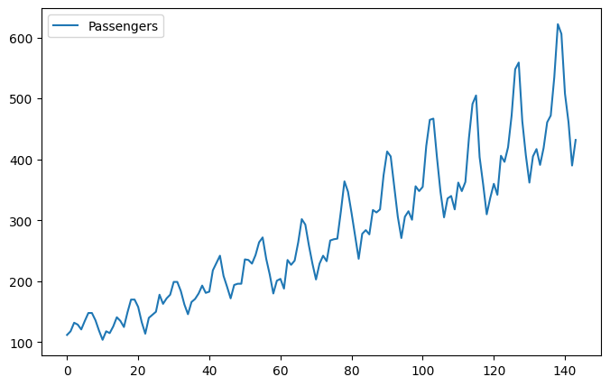
We can see an upward trend over time, and some periodicity that could correspond to vacation periods during the year.
Preprocessing the Data
Let’s now perform some simple preprocessing on the dataset.
First, ensure that all the values in the dataset are expressed as floats (and not integers).
dataset = df.values
dataset = dataset.astype("float32")
Next, normalize the dataset to be in the interval \([0, 1]\).
from sklearn.preprocessing import MinMaxScaler

scaler = MinMaxScaler(feature_range=(0, 1))
dataset = scaler.fit_transform(dataset)
We will use 80% of the data for training and the other 20% for testing.
train_size = int(len(dataset) * 0.8)
test_size = len(dataset) - train_size
train, test = dataset[0:train_size, :], dataset[train_size : len(dataset), :]

print(len(train), len(test))
115 29
We want to provide the model some past data (specifically, LOOK_BACK days worth of data) and then ask it to predict the following day’s passenger count.
LOOK_BACK = 3
import numpy as np


def create_dataset(dataset, look_back=1):
    x, y = [], []
    for i in range(len(dataset) - look_back - 1):
        a = dataset[i : i + look_back, 0]
        x.append(a)
        y.append(dataset[i + look_back, 0])
    return np.array(x), np.array(y)


train_X, train_Y = create_dataset(train, LOOK_BACK)
test_X, test_Y = create_dataset(test, LOOK_BACK)
Keras RNNs require the input to be of the shape (batch, timesteps, features), so we will reshape the input to match this. Since we are just using the passenger counts, we only have one feature to include.
train_X = train_X.reshape(train_X.shape[0], train_X.shape[1], 1)
test_X = test_X.reshape(test_X.shape[0], test_X.shape[1], 1)
Gated Recurrent Unit (GRU) Model
The GRU is an alternative to the traditional Long Short-Term Memory (LSTM) unit. Despite having a much simpler structure than LSTMs, the performance of GRUs are comparable to LSTMs. The implementation of GRUs in Keras-MML also lends them to being easily parallelized, hence improving the speed of training.
import keras
import keras_mml
2024-06-25 05:53:23.247541: I external/local_tsl/tsl/cuda/cudart_stub.cc:32] Could not find cuda drivers on your machine, GPU will not be used.
2024-06-25 05:53:23.249875: I external/local_tsl/tsl/cuda/cudart_stub.cc:32] Could not find cuda drivers on your machine, GPU will not be used.
2024-06-25 05:53:23.280623: I tensorflow/core/platform/cpu_feature_guard.cc:210] This TensorFlow binary is optimized to use available CPU instructions in performance-critical operations.
To enable the following instructions: AVX2 FMA, in other operations, rebuild TensorFlow with the appropriate compiler flags.
2024-06-25 05:53:24.158481: W tensorflow/compiler/tf2tensorrt/utils/py_utils.cc:38] TF-TRT Warning: Could not find TensorRT
The GRU model architecture that we will be using is very rudimentary: we just attach a Dense head to the GRUMML layer for the prediction output. We will aim to minimise MSE loss using the Adam optimizer.
model = keras.Sequential()
model.add(keras.Input((LOOK_BACK, 1)))
model.add(keras_mml.layers.GRUMML(4))
model.add(keras.layers.Dense(1))

model.compile(loss="mse", optimizer="adam", metrics=["mae"])
We define a callback to print the training output once every 10 epochs. This is to reduce clutter on the screen.
class print_training_results_Callback(keras.callbacks.Callback):
    def on_epoch_end(self, epoch, logs=None):
        if int(epoch) % 10 == 0:
            print(
                f"Epoch: {epoch:>3}"
                + f" | loss: {logs['loss']:.5f}"
                + f" | mae: {logs['mae']:.5f}"
                + f" | val_loss: {logs['val_loss']:.5f}"
                + f" | val_mae: {logs['val_mae']:.5f}"
            )
With all that setup, we can train the model!
model.fit(
    train_X,
    train_Y,
    epochs=200,
    batch_size=1,
    validation_split=0.2,
    callbacks=[
        keras.callbacks.EarlyStopping(monitor="val_loss", patience=20, min_delta=1e-4, verbose=1),
        print_training_results_Callback(),
    ],
    verbose=0,
)
Epoch:   0 | loss: 0.08052 | mae: 0.24688 | val_loss: 0.18739 | val_mae: 0.42108
Epoch:  10 | loss: 0.01660 | mae: 0.10555 | val_loss: 0.09703 | val_mae: 0.29545
Epoch:  20 | loss: 0.01445 | mae: 0.09857 | val_loss: 0.08495 | val_mae: 0.27589
Epoch:  30 | loss: 0.00859 | mae: 0.07354 | val_loss: 0.03902 | val_mae: 0.17966
Epoch:  40 | loss: 0.00277 | mae: 0.03970 | val_loss: 0.00928 | val_mae: 0.07497
Epoch:  50 | loss: 0.00219 | mae: 0.03642 | val_loss: 0.00566 | val_mae: 0.06147
Epoch:  60 | loss: 0.00211 | mae: 0.03706 | val_loss: 0.00558 | val_mae: 0.06116
Epoch:  70 | loss: 0.00213 | mae: 0.03738 | val_loss: 0.00525 | val_mae: 0.05992
Epoch:  80 | loss: 0.00208 | mae: 0.03610 | val_loss: 0.00513 | val_mae: 0.05917
Epoch 86: early stopping
<keras.src.callbacks.history.History at 0x7f9c70144a60>
How did the model do?
from sklearn.metrics import mean_squared_error

# Make predictions
train_pred = model.predict(train_X)
test_pred = model.predict(test_X)

# Un-normalize the predictions
train_pred_orig = scaler.inverse_transform(train_pred)
train_Y_orig = scaler.inverse_transform([train_Y])
test_pred_orig = scaler.inverse_transform(test_pred)
test_y_orig = scaler.inverse_transform([test_Y])

# Then evaluate the MSE
train_score = np.sqrt(mean_squared_error(train_Y_orig[0], train_pred_orig[:, 0]))
print(f"Train MSE: {train_score:.2f}")
test_score = np.sqrt(mean_squared_error(test_y_orig[0], test_pred_orig[:, 0]))
print(f"Test MSE:  {test_score:.2f}")
4/4 ━━━━━━━━━━━━━━━━━━━━ 0s 71ms/step
1/1 ━━━━━━━━━━━━━━━━━━━━ 0s 13ms/step
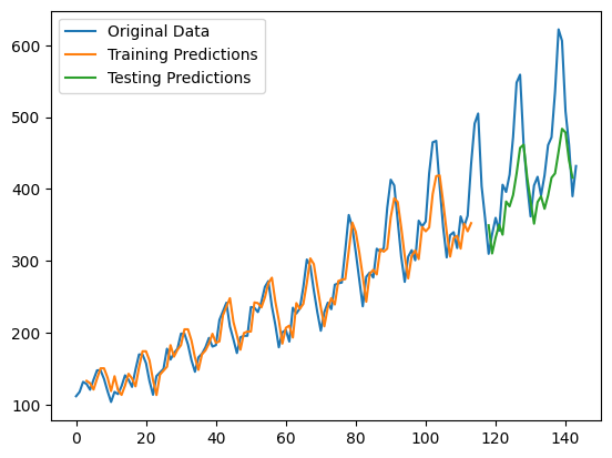
Train MSE: 26.79
Test MSE: 68.21
Let’s also see how the predictions look like.
# Shift train predictions for plotting
train_pred_plot = np.empty_like(dataset)
train_pred_plot[:, :] = np.nan
train_pred_plot[LOOK_BACK : len(train_pred) + LOOK_BACK, :] = train_pred_orig

# Shift test predictions for plotting
test_pred_plot = np.empty_like(dataset)
test_pred_plot[:, :] = np.nan
test_pred_plot[len(train_pred) + (LOOK_BACK * 2) + 1 : len(dataset) - 1, :] = test_pred_orig

# Plot the baselines and the predictions
plt.plot(scaler.inverse_transform(dataset), label="Original Data")
plt.plot(train_pred_plot, label="Training Predictions")
plt.plot(test_pred_plot, label="Testing Predictions")
plt.legend()
plt.show()
Linear Recurrent Unit (LRU) Model
Resurrecting Recurrent Neural Networks for Long Sequences by Orvieto et al. introduces an alternative to the GRU — the LRU. It essentially uses two linear matrix recurrence relations to mimic recurrent units using complex numbers, and this lends it to be easily implemented using regular Dense (and thus the Keras-MML DenseMML) layers.
The architecture of the LRU model is similar to that of the GRU model above, except that we specify the state dimension, which we will take to be 8 here.
model = keras.Sequential()
model.add(keras.Input((LOOK_BACK, 1)))
model.add(keras_mml.layers.LRUMML(4, 8))
model.add(keras.layers.Dense(1))

model.compile(loss="mse", optimizer="adam", metrics=["mae"])
model.fit(
    train_X,
    train_Y,
    epochs=200,
    batch_size=1,
    validation_split=0.2,
    callbacks=[
        keras.callbacks.EarlyStopping(monitor="val_loss", patience=20, min_delta=1e-4, verbose=1),
        print_training_results_Callback(),
    ],
    verbose=0,
)
Epoch:   0 | loss: 0.00472 | mae: 0.05091 | val_loss: 0.01350 | val_mae: 0.09610
Epoch:  10 | loss: 0.00227 | mae: 0.03942 | val_loss: 0.00566 | val_mae: 0.06247
Epoch:  20 | loss: 0.00208 | mae: 0.03701 | val_loss: 0.00592 | val_mae: 0.06309
Epoch:  30 | loss: 0.00205 | mae: 0.03660 | val_loss: 0.00621 | val_mae: 0.06460
Epoch:  40 | loss: 0.00257 | mae: 0.03927 | val_loss: 0.00563 | val_mae: 0.06200
Epoch 46: early stopping
<keras.src.callbacks.history.History at 0x7f9c106a7e20>
We now evaluate the LRU model.
# Make predictions
train_pred = model.predict(train_X)
test_pred = model.predict(test_X)

# Un-normalize the predictions
train_pred_orig = scaler.inverse_transform(train_pred)
train_Y_orig = scaler.inverse_transform([train_Y])
test_pred_orig = scaler.inverse_transform(test_pred)
test_y_orig = scaler.inverse_transform([test_Y])

# Then evaluate the MSE
train_score = np.sqrt(mean_squared_error(train_Y_orig[0], train_pred_orig[:, 0]))
print(f"Train MSE: {train_score:.2f}")
test_score = np.sqrt(mean_squared_error(test_y_orig[0], test_pred_orig[:, 0]))
print(f"Test MSE:  {test_score:.2f}")
4/4 ━━━━━━━━━━━━━━━━━━━━ 0s 82ms/step
1/1 ━━━━━━━━━━━━━━━━━━━━ 0s 14ms/step
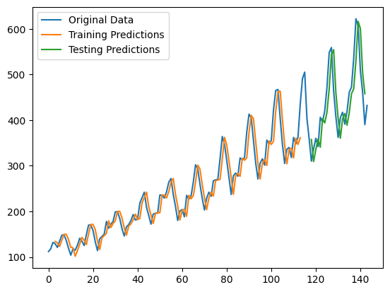
Train MSE: 26.60
Test MSE: 51.00
What does the LRU’s predictions look like?
# Shift train predictions for plotting
train_pred_plot = np.empty_like(dataset)
train_pred_plot[:, :] = np.nan
train_pred_plot[LOOK_BACK : len(train_pred) + LOOK_BACK, :] = train_pred_orig

# Shift test predictions for plotting
test_pred_plot = np.empty_like(dataset)
test_pred_plot[:, :] = np.nan
test_pred_plot[len(train_pred) + (LOOK_BACK * 2) + 1 : len(dataset) - 1, :] = test_pred_orig

# Plot the baselines and the predictions
plt.plot(scaler.inverse_transform(dataset), label="Original Data")
plt.plot(train_pred_plot, label="Training Predictions")
plt.plot(test_pred_plot, label="Testing Predictions")
plt.legend()
plt.show()
Conclusion
In this notebook, we demonstrated how to use Keras-MML’s GRUMML and LRUMML for time series forecasting. They act as suitable replacements for the traditional LSTM layer, and they use dramatically less matrix multiplication operations than normal.