Gated Linear Units (GLUs)

Ryan Kan

Jun 19, 2024

6 min read

In this example, we will explore the use of GLUs, and see how to use Keras-MML’s version of GLUs (i.e., GLUMML).

Note

For the last part of the notebook, we will be using some plotting utilities. You are free to skip them if you want; otherwise, these additional dependencies are required.

%pip install matplotlib~=3.9.0 seaborn~=0.13.2

Requirement already satisfied: matplotlib~=3.9.0 in /home/vscode/.cache/pypoetry/virtualenvs/keras-matmulless-b9IALFmu-py3.10/lib/python3.10/site-packages (3.9.0)
Requirement already satisfied: seaborn~=0.13.2 in /home/vscode/.cache/pypoetry/virtualenvs/keras-matmulless-b9IALFmu-py3.10/lib/python3.10/site-packages (0.13.2)
Requirement already satisfied: contourpy>=1.0.1 in /home/vscode/.cache/pypoetry/virtualenvs/keras-matmulless-b9IALFmu-py3.10/lib/python3.10/site-packages (from matplotlib~=3.9.0) (1.2.1)
Requirement already satisfied: cycler>=0.10 in /home/vscode/.cache/pypoetry/virtualenvs/keras-matmulless-b9IALFmu-py3.10/lib/python3.10/site-packages (from matplotlib~=3.9.0) (0.12.1)
Requirement already satisfied: fonttools>=4.22.0 in /home/vscode/.cache/pypoetry/virtualenvs/keras-matmulless-b9IALFmu-py3.10/lib/python3.10/site-packages (from matplotlib~=3.9.0) (4.53.0)
Requirement already satisfied: kiwisolver>=1.3.1 in /home/vscode/.cache/pypoetry/virtualenvs/keras-matmulless-b9IALFmu-py3.10/lib/python3.10/site-packages (from matplotlib~=3.9.0) (1.4.5)
Requirement already satisfied: numpy>=1.23 in /home/vscode/.cache/pypoetry/virtualenvs/keras-matmulless-b9IALFmu-py3.10/lib/python3.10/site-packages (from matplotlib~=3.9.0) (1.26.4)
Requirement already satisfied: packaging>=20.0 in /home/vscode/.cache/pypoetry/virtualenvs/keras-matmulless-b9IALFmu-py3.10/lib/python3.10/site-packages (from matplotlib~=3.9.0) (24.1)
Requirement already satisfied: pillow>=8 in /home/vscode/.cache/pypoetry/virtualenvs/keras-matmulless-b9IALFmu-py3.10/lib/python3.10/site-packages (from matplotlib~=3.9.0) (10.3.0)
Requirement already satisfied: pyparsing>=2.3.1 in /home/vscode/.cache/pypoetry/virtualenvs/keras-matmulless-b9IALFmu-py3.10/lib/python3.10/site-packages (from matplotlib~=3.9.0) (3.1.2)
Requirement already satisfied: python-dateutil>=2.7 in /home/vscode/.cache/pypoetry/virtualenvs/keras-matmulless-b9IALFmu-py3.10/lib/python3.10/site-packages (from matplotlib~=3.9.0) (2.9.0.post0)
Requirement already satisfied: pandas>=1.2 in /home/vscode/.cache/pypoetry/virtualenvs/keras-matmulless-b9IALFmu-py3.10/lib/python3.10/site-packages (from seaborn~=0.13.2) (2.2.2)
Requirement already satisfied: pytz>=2020.1 in /home/vscode/.cache/pypoetry/virtualenvs/keras-matmulless-b9IALFmu-py3.10/lib/python3.10/site-packages (from pandas>=1.2->seaborn~=0.13.2) (2024.1)
Requirement already satisfied: tzdata>=2022.7 in /home/vscode/.cache/pypoetry/virtualenvs/keras-matmulless-b9IALFmu-py3.10/lib/python3.10/site-packages (from pandas>=1.2->seaborn~=0.13.2) (2024.1)
Requirement already satisfied: six>=1.5 in /home/vscode/.cache/pypoetry/virtualenvs/keras-matmulless-b9IALFmu-py3.10/lib/python3.10/site-packages (from python-dateutil>=2.7->matplotlib~=3.9.0) (1.16.0)

[notice] A new release of pip is available: 24.0 -> 24.1
[notice] To update, run: pip install --upgrade pip
Note: you may need to restart the kernel to use updated packages.

An Introduction to GLUs

In Language Modeling with Gated Convolutional Networks by Dauphin et al., they introduced GLUs, attempting to replace recurrent connections commonly found in Recurrent Neural Networks (RNNs) with gated temporal connections. The idea behind GLUs is simple: we want the neural network to moderate how much information should flow through a given path, like a logical gate.

Suppose the information that ‘wants’ to flow through the network is represented by the vector \(\mathbf{x}\). We moderate the amount of information that is retained by the network by multiplying \(\mathbf{x}\) by a constant, say \(\alpha\), that is bounded in the interval \([0, 1]\). In particular, when \(\alpha = 0\), no information passes through the network, and when \(\alpha = 1\) all the information stored in \(\mathbf{x}\) passes through.

Now we want the network to also learn how much information to flow through the network, i.e. we want the network to also learn this proposed coefficient \(\alpha\). To do so, we could use a Dense layer to learn \(\alpha\), but we need to make sure that the values produced from this step stay in the interval \([0, 1]\). That’s why Dauphin et al. proposes applying the sigmoid activation to this particular layer, in order to bound the coefficient within \([0, 1]\).

In the aforementioned paper, the hidden layers are calculated using

\[ h_l(\mathbf{x}) = (\mathbf{x}\mathbf{W} + \mathbf{b}) \otimes \sigma\left(\mathbf{x}\mathbf{V} + \mathbf{c}\right) \]

where \(\mathbf{x}\) is the input of the layer \(h_l\), the matrices \(\mathbf{W}, \mathbf{V}\) are weights to be learned by the network, \(\mathbf{b}, \mathbf{c}\) are bias vectors that are to also be learned by the network, \(\sigma\) is the sigmoid function, and \(\otimes\) is the element-wise product between matrices.

Of course, there’s no reason why we are restricting ourselves to the sigmoid activation function. In GLU Variants Improve Transformer by Shazeer, they propose alternative activation functions, creating other GLU variants:

\[\begin{split} \begin{align*} \mathrm{ReGLU}(\mathbf{x}, \mathbf{W}, \mathbf{V}, \mathbf{b}, \mathbf{c}) &= \max\left(0, \mathbf{x}\mathbf{W} + \mathbf{b}\right) \otimes (\mathbf{x}\mathbf{V} + \mathbf{c})\\ \mathrm{GEGLU}(\mathbf{x}, \mathbf{W}, \mathbf{V}, \mathbf{b}, \mathbf{c}) &= \mathrm{GELU}\left(0, \mathbf{x}\mathbf{W} + \mathbf{b}\right) \otimes (\mathbf{x}\mathbf{V} + \mathbf{c})\\ \mathrm{SwiGLU}(\mathbf{x}, \mathbf{W}, \mathbf{V}, \mathbf{b}, \mathbf{c}, \beta) &= \mathrm{Swish}_\beta\left(0, \mathbf{x}\mathbf{W} + \mathbf{b}\right) \otimes (\mathbf{x}\mathbf{V} + \mathbf{c})\\ \mathrm{SeGLU}(\mathbf{x}, \mathbf{W}, \mathbf{V}, \mathbf{b}, \mathbf{c}) &= \mathrm{SELU}\left(0, \mathbf{x}\mathbf{W} + \mathbf{b}\right) \otimes (\mathbf{x}\mathbf{V} + \mathbf{c}) \end{align*} \end{split}\]

Note

The \(\mathrm{Swish}_1\) activation function (where \(\beta = 1\)) is equivalent to the \(\mathrm{SiLU}\) (Sigmoid Linear Unit) activation function.

A Simple Example With GLUs

To demonstrate the use of GLUs, we make a simple dataset with the following rules.

1. Each feature vector is a 5-dimensional vector. For example, [1, 0, 1, 0, 1].

2. If the first and third entries sum to at least 1, the output will be the input divided by 2. For example, [1, 0, 1, 0, 1] becomes [0.5, 0, 0.5, 0., 0.5].

3. Otherwise the output will all be zeroes. For example [0, 1, 0, 1, 0] becomes [0, 0, 0, 0, 0].

We create a dataset of 10000 entries.

import numpy as np

np.random.seed(42)  # For reproducibility

X = np.random.uniform(low=0, size=(10000, 5))

y = np.zeros_like(X)
condition = X[:, 0] + X[:, 2] >= 1
indices = np.where(condition)
y[indices] = X[indices] * 0.5

print(X[:5])
print(y[:5])

[[0.37454012 0.95071431 0.73199394 0.59865848 0.15601864]
 [0.15599452 0.05808361 0.86617615 0.60111501 0.70807258]
 [0.02058449 0.96990985 0.83244264 0.21233911 0.18182497]
 [0.18340451 0.30424224 0.52475643 0.43194502 0.29122914]
 [0.61185289 0.13949386 0.29214465 0.36636184 0.45606998]]
[[0.18727006 0.47535715 0.36599697 0.29932924 0.07800932]
 [0.07799726 0.02904181 0.43308807 0.30055751 0.35403629]
 [0.         0.         0.         0.         0.        ]
 [0.         0.         0.         0.         0.        ]
 [0.         0.         0.         0.         0.        ]]

We use a train-test split of 9:1.

train_data = X[:9000], y[:9000]
test_data = X[9000:], y[9000:]

The model that we will use is the traditional GLU model with the sigmoid activation function.

import keras

import keras_mml

2024-06-25 03:00:04.993881: I external/local_tsl/tsl/cuda/cudart_stub.cc:32] Could not find cuda drivers on your machine, GPU will not be used.
2024-06-25 03:00:04.996054: I external/local_tsl/tsl/cuda/cudart_stub.cc:32] Could not find cuda drivers on your machine, GPU will not be used.
2024-06-25 03:00:05.024675: I tensorflow/core/platform/cpu_feature_guard.cc:210] This TensorFlow binary is optimized to use available CPU instructions in performance-critical operations.
To enable the following instructions: AVX2 FMA, in other operations, rebuild TensorFlow with the appropriate compiler flags.
2024-06-25 03:00:05.726507: W tensorflow/compiler/tf2tensorrt/utils/py_utils.cc:38] TF-TRT Warning: Could not find TensorRT

model = keras.Sequential(
    layers=[
        keras.layers.Input(shape=(5,)),
        keras_mml.layers.GLUMML(32, activation="sigmoid"),
        keras.layers.Dense(5)
    ], 
    name="GLU-Model"
)
model.compile(
    loss="mse",
    optimizer="adam",
    metrics=["mae"]
)
model.summary()

Model: "GLU-Model"

┏━━━━━━━━━━━━━━━━━━━━━━━━━━━━━━━━━┳━━━━━━━━━━━━━━━━━━━━━━━━┳━━━━━━━━━━━━━━━┓
┃ Layer (type)                    ┃ Output Shape           ┃       Param # ┃
┡━━━━━━━━━━━━━━━━━━━━━━━━━━━━━━━━━╇━━━━━━━━━━━━━━━━━━━━━━━━╇━━━━━━━━━━━━━━━┩
│ glumml (GLUMML)                 │ (None, 32)             │        11,296 │
├─────────────────────────────────┼────────────────────────┼───────────────┤
│ dense (Dense)                   │ (None, 5)              │           165 │
└─────────────────────────────────┴────────────────────────┴───────────────┘

 Total params: 11,461 (44.77 KB)

 Trainable params: 11,461 (44.77 KB)

 Non-trainable params: 0 (0.00 B)

We define a callback to print the training output once every 10 epochs. This is to reduce clutter on the screen.

class print_training_results_Callback(keras.callbacks.Callback):
    def on_epoch_end(self, epoch, logs=None):
        if int(epoch) % 10 == 0:
            print(
                f"Epoch: {epoch:>3}"
                + f" | loss: {logs['loss']:.5f}"
                + f" | mae: {logs['mae']:.5f}"
                + f" | val_loss: {logs['val_loss']:.5f}"
                + f" | val_mae: {logs['val_mae']:.5f}"
            )

Now we can train the model. We train it for 100 epochs using a batch size of 256.

NUM_EPOCHS = 100
BATCH_SIZE = 256

history = model.fit(
    train_data[0],
    train_data[1],
    validation_data=test_data,
    epochs=NUM_EPOCHS,
    batch_size=BATCH_SIZE,
    verbose=0,
    callbacks=[print_training_results_Callback()]
)

Epoch:   0 | loss: 0.03405 | mae: 0.14737 | val_loss: 0.02811 | val_mae: 0.15123
Epoch:  10 | loss: 0.01461 | mae: 0.09357 | val_loss: 0.01411 | val_mae: 0.09278
Epoch:  20 | loss: 0.01438 | mae: 0.09166 | val_loss: 0.01437 | val_mae: 0.09324
Epoch:  30 | loss: 0.01405 | mae: 0.08971 | val_loss: 0.01388 | val_mae: 0.08902
Epoch:  40 | loss: 0.01395 | mae: 0.08884 | val_loss: 0.01311 | val_mae: 0.08603
Epoch:  50 | loss: 0.01391 | mae: 0.08841 | val_loss: 0.01363 | val_mae: 0.08741
Epoch:  60 | loss: 0.01392 | mae: 0.08811 | val_loss: 0.01305 | val_mae: 0.08547
Epoch:  70 | loss: 0.01375 | mae: 0.08711 | val_loss: 0.01300 | val_mae: 0.08499
Epoch:  80 | loss: 0.01387 | mae: 0.08725 | val_loss: 0.01290 | val_mae: 0.08477
Epoch:  90 | loss: 0.01370 | mae: 0.08639 | val_loss: 0.01351 | val_mae: 0.08611

test_mse, test_mae = model.evaluate(test_data[0], test_data[1])
print("Test MSE:", test_mse)
print("Test MAE:", test_mae)

32/32 ━━━━━━━━━━━━━━━━━━━━ 0s 767us/step - loss: 0.0124 - mae: 0.0819
Test MSE: 0.01287087518721819
Test MAE: 0.08368378132581711

Let’s save the record of validation losses for later, so we can make a comparison between different GLU variants.

validation_losses = {}
validation_losses["GLU"] = history.history["val_loss"]

Other GLU Variants

Let’s also try out the GLUMML layer on different GLU variants.

VARIANT_MAP = {
    "Bilinear": "linear",
    "GEGLU": "gelu",
    "ReGLU": "relu",
    "SwiGLU": "silu",  # Silu is the same as Swish when beta = 1
    "SeGLU": "selu"
}

def train_variant(variant_name):
    print(f" {variant_name} ".center(50, "="))
    activation_func = VARIANT_MAP[variant_name]
    
    model = keras.Sequential(
        layers=[
            keras.layers.Input(shape=(5,)),
            keras_mml.layers.GLUMML(32, activation=activation_func),
            keras.layers.Dense(5)
        ], 
        name=f"{variant_name}-Model"
    )
    model.compile(
        loss="mse",
        optimizer="adam",
        metrics=["mae"]
    )
    
    history = model.fit(
        train_data[0],
        train_data[1],
        validation_data=test_data,
        epochs=NUM_EPOCHS,
        batch_size=BATCH_SIZE,
        verbose=0,
        callbacks=[print_training_results_Callback()]
    )
    
    validation_losses[variant_name] = history.history["val_loss"]
    print()

for variant in VARIANT_MAP:
    train_variant(variant)

==================== Bilinear ====================
Epoch:   0 | loss: 0.03370 | mae: 0.14422 | val_loss: 0.02658 | val_mae: 0.14571
Epoch:  10 | loss: 0.01266 | mae: 0.07863 | val_loss: 0.01249 | val_mae: 0.07699
Epoch:  20 | loss: 0.01230 | mae: 0.07588 | val_loss: 0.01169 | val_mae: 0.07430
Epoch:  30 | loss: 0.01221 | mae: 0.07551 | val_loss: 0.01163 | val_mae: 0.07511
Epoch:  40 | loss: 0.01211 | mae: 0.07475 | val_loss: 0.01194 | val_mae: 0.07606
Epoch:  50 | loss: 0.01209 | mae: 0.07459 | val_loss: 0.01199 | val_mae: 0.07541
Epoch:  60 | loss: 0.01200 | mae: 0.07439 | val_loss: 0.01158 | val_mae: 0.07330
Epoch:  70 | loss: 0.01192 | mae: 0.07400 | val_loss: 0.01133 | val_mae: 0.07218
Epoch:  80 | loss: 0.01197 | mae: 0.07416 | val_loss: 0.01116 | val_mae: 0.07150
Epoch:  90 | loss: 0.01188 | mae: 0.07413 | val_loss: 0.01115 | val_mae: 0.07171

===================== GEGLU ======================
Epoch:   0 | loss: 0.03455 | mae: 0.14384 | val_loss: 0.02646 | val_mae: 0.14400
Epoch:  10 | loss: 0.01270 | mae: 0.07863 | val_loss: 0.01188 | val_mae: 0.07551
Epoch:  20 | loss: 0.01246 | mae: 0.07710 | val_loss: 0.01149 | val_mae: 0.07400
Epoch:  30 | loss: 0.01227 | mae: 0.07588 | val_loss: 0.01130 | val_mae: 0.07170
Epoch:  40 | loss: 0.01218 | mae: 0.07554 | val_loss: 0.01154 | val_mae: 0.07336
Epoch:  50 | loss: 0.01218 | mae: 0.07535 | val_loss: 0.01147 | val_mae: 0.07285
Epoch:  60 | loss: 0.01206 | mae: 0.07494 | val_loss: 0.01140 | val_mae: 0.07227
Epoch:  70 | loss: 0.01198 | mae: 0.07453 | val_loss: 0.01124 | val_mae: 0.07227
Epoch:  80 | loss: 0.01196 | mae: 0.07415 | val_loss: 0.01136 | val_mae: 0.07228
Epoch:  90 | loss: 0.01192 | mae: 0.07373 | val_loss: 0.01135 | val_mae: 0.07187

===================== ReGLU ======================
Epoch:   0 | loss: 0.03449 | mae: 0.14628 | val_loss: 0.02701 | val_mae: 0.14630
Epoch:  10 | loss: 0.01278 | mae: 0.08074 | val_loss: 0.01228 | val_mae: 0.07942
Epoch:  20 | loss: 0.01216 | mae: 0.07524 | val_loss: 0.01175 | val_mae: 0.07349
Epoch:  30 | loss: 0.01224 | mae: 0.07445 | val_loss: 0.01144 | val_mae: 0.07310
Epoch:  40 | loss: 0.01191 | mae: 0.07275 | val_loss: 0.01116 | val_mae: 0.07187
Epoch:  50 | loss: 0.01175 | mae: 0.07213 | val_loss: 0.01103 | val_mae: 0.06993
Epoch:  60 | loss: 0.01174 | mae: 0.07122 | val_loss: 0.01109 | val_mae: 0.07001
Epoch:  70 | loss: 0.01180 | mae: 0.07197 | val_loss: 0.01176 | val_mae: 0.07116
Epoch:  80 | loss: 0.01166 | mae: 0.07153 | val_loss: 0.01129 | val_mae: 0.07042
Epoch:  90 | loss: 0.01172 | mae: 0.07183 | val_loss: 0.01117 | val_mae: 0.07387

===================== SwiGLU =====================
Epoch:   0 | loss: 0.03258 | mae: 0.14407 | val_loss: 0.02543 | val_mae: 0.14162
Epoch:  10 | loss: 0.01272 | mae: 0.07913 | val_loss: 0.01196 | val_mae: 0.07712
Epoch:  20 | loss: 0.01251 | mae: 0.07735 | val_loss: 0.01169 | val_mae: 0.07421
Epoch:  30 | loss: 0.01238 | mae: 0.07678 | val_loss: 0.01148 | val_mae: 0.07436
Epoch:  40 | loss: 0.01215 | mae: 0.07537 | val_loss: 0.01153 | val_mae: 0.07451
Epoch:  50 | loss: 0.01217 | mae: 0.07577 | val_loss: 0.01140 | val_mae: 0.07281
Epoch:  60 | loss: 0.01202 | mae: 0.07483 | val_loss: 0.01135 | val_mae: 0.07214
Epoch:  70 | loss: 0.01202 | mae: 0.07458 | val_loss: 0.01196 | val_mae: 0.07468
Epoch:  80 | loss: 0.01192 | mae: 0.07416 | val_loss: 0.01152 | val_mae: 0.07381
Epoch:  90 | loss: 0.01183 | mae: 0.07413 | val_loss: 0.01116 | val_mae: 0.07045

===================== SeGLU ======================
Epoch:   0 | loss: 0.03265 | mae: 0.14473 | val_loss: 0.02602 | val_mae: 0.14425
Epoch:  10 | loss: 0.01261 | mae: 0.07809 | val_loss: 0.01206 | val_mae: 0.07636
Epoch:  20 | loss: 0.01232 | mae: 0.07644 | val_loss: 0.01175 | val_mae: 0.07499
Epoch:  30 | loss: 0.01208 | mae: 0.07450 | val_loss: 0.01174 | val_mae: 0.07386
Epoch:  40 | loss: 0.01198 | mae: 0.07378 | val_loss: 0.01182 | val_mae: 0.07710
Epoch:  50 | loss: 0.01191 | mae: 0.07378 | val_loss: 0.01125 | val_mae: 0.07215
Epoch:  60 | loss: 0.01201 | mae: 0.07413 | val_loss: 0.01166 | val_mae: 0.07526
Epoch:  70 | loss: 0.01193 | mae: 0.07372 | val_loss: 0.01131 | val_mae: 0.07064
Epoch:  80 | loss: 0.01190 | mae: 0.07347 | val_loss: 0.01108 | val_mae: 0.06964
Epoch:  90 | loss: 0.01177 | mae: 0.07279 | val_loss: 0.01146 | val_mae: 0.07267

Comparison Models

Let’s also define two comparison models to assess against the GLU models.

The first will be a simple MLP that uses a \(\mathrm{Sigmoid}\) activation in the middle layer.

model = keras.Sequential(
    layers=[
        keras.layers.Input(shape=(5,)),
        keras_mml.layers.DenseMML(32),
        keras_mml.layers.DenseMML(256, activation="sigmoid"),
        keras_mml.layers.DenseMML(32),
        keras.layers.Dense(5)
    ], 
    name="Dense-With-Sigmoid-Model"
)
model.compile(
    loss="mse",
    optimizer="adam",
    metrics=["mae"]
)
model.summary()

Model: "Dense-With-Sigmoid-Model"

┏━━━━━━━━━━━━━━━━━━━━━━━━━━━━━━━━━┳━━━━━━━━━━━━━━━━━━━━━━━━┳━━━━━━━━━━━━━━━┓
┃ Layer (type)                    ┃ Output Shape           ┃       Param # ┃
┡━━━━━━━━━━━━━━━━━━━━━━━━━━━━━━━━━╇━━━━━━━━━━━━━━━━━━━━━━━━╇━━━━━━━━━━━━━━━┩
│ dense_mml_12 (DenseMML)         │ (None, 32)             │           192 │
├─────────────────────────────────┼────────────────────────┼───────────────┤
│ dense_mml_13 (DenseMML)         │ (None, 256)            │         8,448 │
├─────────────────────────────────┼────────────────────────┼───────────────┤
│ dense_mml_14 (DenseMML)         │ (None, 32)             │         8,224 │
├─────────────────────────────────┼────────────────────────┼───────────────┤
│ dense_6 (Dense)                 │ (None, 5)              │           165 │
└─────────────────────────────────┴────────────────────────┴───────────────┘

 Total params: 17,029 (66.52 KB)

 Trainable params: 17,029 (66.52 KB)

 Non-trainable params: 0 (0.00 B)

history = model.fit(
    train_data[0],
    train_data[1],
    validation_data=test_data,
    epochs=NUM_EPOCHS,
    batch_size=BATCH_SIZE,
    verbose=0,
    callbacks=[print_training_results_Callback()]
)
validation_losses["Dense-With-Sigmoid"] = history.history["val_loss"]

Epoch:   0 | loss: 0.03580 | mae: 0.14715 | val_loss: 0.02941 | val_mae: 0.15550
Epoch:  10 | loss: 0.02913 | mae: 0.15220 | val_loss: 0.02877 | val_mae: 0.15167
Epoch:  20 | loss: 0.02187 | mae: 0.11718 | val_loss: 0.02164 | val_mae: 0.12403
Epoch:  30 | loss: 0.01942 | mae: 0.10809 | val_loss: 0.01865 | val_mae: 0.10386
Epoch:  40 | loss: 0.01838 | mae: 0.10359 | val_loss: 0.01786 | val_mae: 0.10429
Epoch:  50 | loss: 0.01804 | mae: 0.10337 | val_loss: 0.01782 | val_mae: 0.09880
Epoch:  60 | loss: 0.01729 | mae: 0.09994 | val_loss: 0.01760 | val_mae: 0.10598
Epoch:  70 | loss: 0.01699 | mae: 0.09896 | val_loss: 0.01600 | val_mae: 0.09559
Epoch:  80 | loss: 0.01694 | mae: 0.09897 | val_loss: 0.01628 | val_mae: 0.09480
Epoch:  90 | loss: 0.01679 | mae: 0.09835 | val_loss: 0.01580 | val_mae: 0.09481

The second is similar to the first, but instead of \(\mathrm{Sigmoid}\) we will use \(\mathrm{ReLU}\).

model = keras.Sequential(
    layers=[
        keras.layers.Input(shape=(5,)),
        keras_mml.layers.DenseMML(32),
        keras_mml.layers.DenseMML(256, activation="relu"),
        keras_mml.layers.DenseMML(32),
        keras.layers.Dense(5)
    ], 
    name="Dense-With-ReLU-Model"
)
model.compile(
    loss="mse",
    optimizer="adam",
    metrics=["mae"]
)
model.summary()

Model: "Dense-With-ReLU-Model"

┏━━━━━━━━━━━━━━━━━━━━━━━━━━━━━━━━━┳━━━━━━━━━━━━━━━━━━━━━━━━┳━━━━━━━━━━━━━━━┓
┃ Layer (type)                    ┃ Output Shape           ┃       Param # ┃
┡━━━━━━━━━━━━━━━━━━━━━━━━━━━━━━━━━╇━━━━━━━━━━━━━━━━━━━━━━━━╇━━━━━━━━━━━━━━━┩
│ dense_mml_15 (DenseMML)         │ (None, 32)             │           192 │
├─────────────────────────────────┼────────────────────────┼───────────────┤
│ dense_mml_16 (DenseMML)         │ (None, 256)            │         8,448 │
├─────────────────────────────────┼────────────────────────┼───────────────┤
│ dense_mml_17 (DenseMML)         │ (None, 32)             │         8,224 │
├─────────────────────────────────┼────────────────────────┼───────────────┤
│ dense_7 (Dense)                 │ (None, 5)              │           165 │
└─────────────────────────────────┴────────────────────────┴───────────────┘

 Total params: 17,029 (66.52 KB)

 Trainable params: 17,029 (66.52 KB)

 Non-trainable params: 0 (0.00 B)

history = model.fit(
    train_data[0],
    train_data[1],
    validation_data=test_data,
    epochs=NUM_EPOCHS,
    batch_size=BATCH_SIZE,
    verbose=0,
    callbacks=[print_training_results_Callback()]
)
validation_losses["Dense-With-ReLU"] = history.history["val_loss"]

Epoch:   0 | loss: 0.03433 | mae: 0.14594 | val_loss: 0.02808 | val_mae: 0.15051
Epoch:  10 | loss: 0.01221 | mae: 0.07438 | val_loss: 0.01189 | val_mae: 0.07238
Epoch:  20 | loss: 0.01136 | mae: 0.06882 | val_loss: 0.01094 | val_mae: 0.06790
Epoch:  30 | loss: 0.01121 | mae: 0.06837 | val_loss: 0.01137 | val_mae: 0.07015
Epoch:  40 | loss: 0.01102 | mae: 0.06781 | val_loss: 0.01150 | val_mae: 0.06923
Epoch:  50 | loss: 0.01106 | mae: 0.06671 | val_loss: 0.01035 | val_mae: 0.06429
Epoch:  60 | loss: 0.01097 | mae: 0.06702 | val_loss: 0.01060 | val_mae: 0.06422
Epoch:  70 | loss: 0.01093 | mae: 0.06614 | val_loss: 0.01052 | val_mae: 0.06362
Epoch:  80 | loss: 0.01080 | mae: 0.06583 | val_loss: 0.01026 | val_mae: 0.06258
Epoch:  90 | loss: 0.01074 | mae: 0.06534 | val_loss: 0.01042 | val_mae: 0.06385

Plotting Losses

Let’s plot the validation losses over time.

import matplotlib.pyplot as plt
import seaborn as sns

plt.figure(figsize=(14, 5), dpi=100)

for variant in validation_losses: 
    sns.lineplot(validation_losses[variant], label=variant)

plt.legend()
plt.yscale("log")
plt.ylabel("Log Loss")
plt.xlabel("Epoch Number")
plt.title("Losses")
plt.tight_layout()

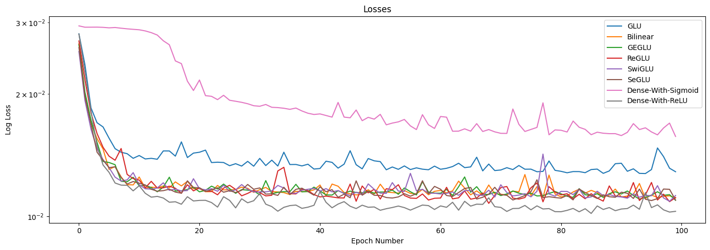
We can’t really see the losses after epoch 20, so let’s zoom into that part specifically. Also, Dense-With-Sigmoid performs very poorly, so let’s exclude that from our analysis below.

plt.figure(figsize=(14, 5), dpi=100)

for variant in validation_losses:
    if variant == "Dense-With-Sigmoid":
        continue
    sns.lineplot(validation_losses[variant][20:], label=variant)

plt.legend()
plt.yscale("log")
plt.ylabel("Log Loss")
plt.xlabel("Epoch Number - 20")
plt.title("Losses After Epoch 20")
plt.tight_layout()

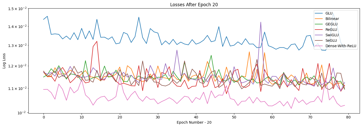
Conclusion

From the charts above, we can conclude that all the different models seem to stabilize pretty quickly. However, it is important to note that this is just a toy example, and that GLUs may have a different performance on real datasets. It is thus important to assess all different kinds of architectures before deciding on one.